Quick start
The Null Space Optimizer is an algorithm that solves arbitrary nonlinear constrained optimization problems of the form
where \(\mathcal{X}\) is the optimization set, \(J\,:\,\mathcal{X}\to \mathbb{R}\) is the objective function, \(g\,:\,\mathcal{X}\rightarrow \mathbb{R}^p\) and \(h\,:\,\mathcal{X}\rightarrow \mathbb{R}^q\) are respectively the equality and inequality constraint functionals. The optimization set \(\mathcal{X}\) may be, but is not restricted to finite-dimensional or even a vector space; it can be rather arbitrary and needs only a sort of manifold structure .
The whole algorithm is described in
[1] Feppon F., Allaire G. and Dapogny C. Null space gradient flows for constrained optimization with applications to shape optimization. 2019. ESAIM: COCV, 26 90 (Open Access). HAL preprint hal-01972915
and its extension to for dealing with many constraints with sparse Jacobian matrix is explained in
[2] Feppon F. Density based topology optimization with the Null Space Optimizer: a tutorial and a comparison (2023). Submitted. HAL preprint hal-04155507.
Solving standard optimization problems
In many “standard” optimization problems, the design variable belong to a finite-dimensional space \(\mathbb{R}^n\) where \(n\) is a fixed integer.
Let us illustrate how to use the Null Space Optimizer to solve the following simple optimization problem based on basic_examples/ex05_multiple_shootings.py:
This problem can be implemented by
instantiating an EuclideanOptimizable object:
from nullspace_optimizer import EuclideanOptimizable

class problemSimple(EuclideanOptimizable):
    # Initialization
    def x0(self):
        return [1.25,0]

    # Objective function
    def J(self, x):
        return (x[0]+1)**2+(x[1]+1)**2

    # Inequality constraint
    def H(self, x):
        return [x[0]**2+x[1]**2-1**2,
                x[0]+x[1]-1,
                -x[1]-0.7]

    # Row vector with the gradient of J
    def dJ(self, x):
        return [2*(x[0]+1), 2*(x[1]+1)]

    # Jacobian matrix of H
    def dH(self, x):
        return [[2*x[0], 2*x[1]],
                [1, 1],
                [0, -1]]
Actually, for this simple problem, the gradient and Jacobian matrix can be computed automatically with symbolic differentiation.
The problem can then be solved numerically with the nlspace_solve() function.
from nullspace_optimizer import nlspace_solve

# dt : the time step
# debug=1 for verbosity
params = {'dt': 0.1}
opt_results = nlspace_solve(problemSimple(), params)
The time step params['dt']=0.01
delimits the maximal update size. Running the following code yields the following output:
0. J=6.0625 G=[] H=[0.5625,0.25,-0.7]
1. J=5.09448 G=[] H=[0.1056,-0.005556,-0.6444]
2. J=4.48126 G=[] H=[-0.156,-0.1814,-0.6049]
3. J=4.09178 G=[] H=[-0.2949,-0.3067,-0.5646]
4. J=3.73614 G=[] H=[-0.4111,-0.4264,-0.5262]
5. J=3.41142 G=[] H=[-0.5071,-0.5407,-0.4895]
6. J=3.11492 G=[] H=[-0.585,-0.65,-0.4544]
7. J=2.84419 G=[] H=[-0.6468,-0.7545,-0.4209]
8. J=2.597 G=[] H=[-0.6944,-0.8543,-0.3888]
9. J=2.37128 G=[] H=[-0.7294,-0.9496,-0.3582]
10. J=2.16518 G=[] H=[-0.7533,-1.041,-0.329]
11. J=1.977 G=[] H=[-0.7673,-1.128,-0.301]
12. J=1.80517 G=[] H=[-0.7727,-1.211,-0.2743]
13. J=1.64828 G=[] H=[-0.7706,-1.291,-0.2488]
14. J=1.50502 G=[] H=[-0.7619,-1.367,-0.2244]
15. J=1.37421 G=[] H=[-0.7475,-1.439,-0.2011]
16. J=1.25478 G=[] H=[-0.7282,-1.509,-0.1788]
17. J=1.14572 G=[] H=[-0.7047,-1.575,-0.1575]
18. J=1.04614 G=[] H=[-0.6776,-1.638,-0.1372]
19. J=0.955217 G=[] H=[-0.6474,-1.699,-0.1178]
20. J=0.872196 G=[] H=[-0.6148,-1.757,-0.0992]
21. J=0.79639 G=[] H=[-0.5801,-1.812,-0.08145]
22. J=0.727173 G=[] H=[-0.5437,-1.865,-0.0645]
23. J=0.663972 G=[] H=[-0.5059,-1.915,-0.0483]
24. J=0.606263 G=[] H=[-0.4672,-1.963,-0.03282]
25. J=0.553571 G=[] H=[-0.4277,-2.009,-0.01803]
26. J=0.505458 G=[] H=[-0.3878,-2.053,-0.003894]
27. J=0.467436 G=[] H=[-0.3617,-2.085,-0.0003894]
28. J=0.434441 G=[] H=[-0.3394,-2.113,-3.894e-05]
29. J=0.404486 G=[] H=[-0.3171,-2.139,-3.894e-06]
30. J=0.377151 G=[] H=[-0.2946,-2.164,-3.894e-07]
31. J=0.352193 G=[] H=[-0.2719,-2.188,-3.894e-08]
32. J=0.329405 G=[] H=[-0.2492,-2.211,-3.894e-09]
33. J=0.308597 G=[] H=[-0.2265,-2.232,-3.894e-10]
34. J=0.289598 G=[] H=[-0.2039,-2.253,-3.894e-11]
35. J=0.272251 G=[] H=[-0.1816,-2.273,-3.894e-12]
36. J=0.256411 G=[] H=[-0.1595,-2.292,-3.895e-13]
37. J=0.241947 G=[] H=[-0.1377,-2.31,-3.897e-14]
38. J=0.228741 G=[] H=[-0.1162,-2.328,-3.886e-15]
39. J=0.216682 G=[] H=[-0.09517,-2.344,-4.441e-16]
40. J=0.205672 G=[] H=[-0.07454,-2.36,0]
41. J=0.195619 G=[] H=[-0.05436,-2.375,0]
42. J=0.186439 G=[] H=[-0.03465,-2.389,0]
43. J=0.178057 G=[] H=[-0.01543,-2.403,0]
44. J=0.172294 G=[] H=[-0.001446,-2.413,0]
45. J=0.171772 G=[] H=[-0.0001437,-2.414,0]
46. J=0.17172 G=[] H=[-1.436e-05,-2.414,0]
47. J=0.171715 G=[] H=[-1.436e-06,-2.414,0]


Optimization completed.
48. J=0.171714 G=[] H=[-1.436e-07,-2.414,0]
For this simple optimization problem with two variables, it is possible to draw the optimization trajectory with
import nullspace_optimizer.examples.basic_examples.utils.draw as draw

draw.drawProblem(problemSimple(), [-1.5, 1.5], [-1.5, 1.5])
draw.drawData(opt_results, f'x0', f'C0', x0=True, xfinal=True, initlabel=None)
draw.show()
which should produce the following figure:

Using the Null Space Optimizer on general optimization sets
It is possible to use the Null Space Optimizer for for more involved applications than parametric optimization working on Euclidean spaces as described above. One of the initial motivations for the development of the Null Space Optimizer was to be used for topology optimization with the level set method (see [1]).
The nlspace_solve() function is designed to
perform optimization on general sets respecting some manifold structure.
These sets must comply with the structure of the Optimizable class
that requires a minimum number of methods to be defined,
that contain all the necessary information about the
optimization problem to solve (objective and constraint functions,
derivatives…).
An Optimizable
object should implement the following structure:
from nullspace_optimizer import Optimizable

class MyOptimizable(Optimizable):
    # Initialization
    def x0(self):
        pass

    # Objective function
    def J(self, x):
        pass

    # Equality constraints
    def G(self, x):
        pass

    # Inequality constraints
    def H(self, x):
        pass

    # Derivative of the objective function
    def dJ(self, x):
        pass

    # Jacobian matrix of G
    def dG(self, x):
        pass

    # Jacobian matrix of H
    def dH(self, x):
        pass

    # Inner product metrizing the optimization set
    def inner_product(self, x):
        pass

    # Retraction
    def retract(self, x, dx):
        pass

    # Post processing every time a
    # point on the optimization path is accepted
    def accept(self, params, results):
        pass
The methods inner_product and retract
are useful to perform optimization on very general optimization sets.
When solving standard optimization problems in \(\mathbb{R}^n\),
with the subclass EuclideanOptimizable, these methods are
defined automatically. If the optimization problem features no equality constraint (respectively, no inequality constraint),
the methods G and dG (respectively H and dH) do not need to be defined.
These methods must satisfy the following requirements:
\(\texttt{J}:\mathcal{X}\to\mathbb{R}\), \(\texttt{G}:\mathcal{X}\to\mathbb{R}^p\), \(\texttt{H}:\mathcal{X}\to\mathbb{R}^q\) objective function, \(p\) equality constraints and \(q\) inequality constraints;
\(\texttt{retract}:\mathcal{X}\times \R^{n}\to \mathcal{X}\): a retraction that converts the current point
xand a tangent vectordx\(\in \R^{n}\) into a new point \(\texttt{retract(x,dx)}\in \mathcal{X}\) on the manifold \(\mathcal{X}\). TheOptimizableobject is conceptually understood as a curved set where one can move from one point to another in a direction from the tangent space. The retraction is a map that allows to do this update. Here, \(n\) is thought of as the dimension of the tangent space of \(\mathcal{X}\) to \(\texttt{x}\in\mathcal{X}\). This tangent space does not need to remain constant along iterations. An illustration of this concept is given in the following figure: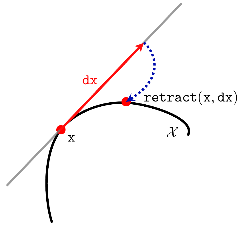
Schematic of the retractmap which allows to perform design updates given the current pointxand the descent directiondx.¶\(\texttt{DJ}:\mathcal{X}\to\mathbb{R}^n\), \(\texttt{DG}:\mathcal{X}\to\mathbb{R}^{p\times n}\), \(\texttt{DH} :\Chi \to \R^{q\times n}\): (Fréchet) derivatives of objective and constraints as functions. This means that the following asymptotic expansion must hold:
\[\texttt{J}(\texttt{retract}(\texttt{x},h\times\texttt{dx}))=\texttt{J}(\texttt{x})+ h \times \texttt{DJ}(\texttt{x})^{T}\texttt{dx} +o(h) \text{ as } h\rightarrow 0,\]and similarly for \(\texttt{DG}\) and \(\texttt{DH}\). In other words, \(\texttt{DJ}^{T}\texttt{dx}\) is the variation of the objective function \(\texttt{J}\) at \(\texttt{x}\) along the tangent direction \(\texttt{dx}\in \mathbb{R}^{n}\).
\(\texttt{inner\_product}:\,\mathcal{X}\to \mathbb{R}^{n\times n}\): the local inner product needed for the computation of gradients, given in the form of a sparse scipy matrix in the csc format. If \(A=\texttt{inner\_product}(\texttt{x})\), then the gradients at \(\texttt{x}\) are given by \(\nabla \texttt{J}(\texttt{x})=A^{-1}\texttt{DJ(x)}\), \(\nabla \texttt{g}_i(\texttt{x}):=A^{-1}\texttt{Dg}_i(\texttt{x})\), \(\nabla\texttt{h}_j(\texttt{x}):=A^{-1}\texttt{Dh}_j(\texttt{x})\). Of course, \(A\) must be a symmetric positive definite matrix.
accept: an optional function that is called by the optimization algorithm when the next point is accepted, which serves e.g. for saving current available information before proceeding to the next iteration. This method has access to theresultsdictionary that contains the output of the optimization as well as the dictionaryparams. These dictionary can be manually updated in the course of the optimization if the user wants to implement gradation schemes.
Note
The variable x from the implementation
does not need at all to be a vector: it can
be for instance the path to a file. Only dx needs to be
a vector (a numpy array).
This programming paradigm allows to use the Null Space Optimizer
on
a variety of applications. For instance, it was used for 3D
topology optimization with various constraints in
[3] Feppon, F., Allaire, G., Dapogny D. and Jolivet, P. Topology optimization of thermal fluid-structure systems using body-fitted meshes and parallel computing (2020). Journal of Computational Physics, 109574. HAL preprint hal-02518207.
Running the Null Space Optimizer
The nlspace_solve() function can run on any
Optimizable that respects the structure described above.
The prototype of this function reads:
from nullspace_optimizer import nlspace_solve

# Define problem

opt_results = nlspace_solve(problem: Optimizable, params=None, results=None)
The input variables are
problem: anOptimizableobject implementing the structure described above. For standard optimization problems sets on Euclidean spaces, it is sufficient to instantiate the subclassEuclideanOptimizable.params: (optional) a dictionary containing algorithm parameters.results: (optional) a previous output of thenlspace_solve()function. If supplied, the optimization will keep going from the last input of the dictionaryresults['x'][-1]. This is useful when one needs to restart an optimization after an interruption.
The optimization routine nlspace_solve() returns the dictionary
opt_results which contains various information about the
optimization path. The optimized variable is accessible via
results['x'][-1].
Basic principles of the algorithm
The basis of the method is to solve an Ordinary Differential Equation (so-called ‘’null-space gradient flow’’),
which is able to solve the optimization problem above.
The direction \(\xi_J(x(t))\) is called the null space direction, it is the ‘’best’’ (in an \(L^2\) sense) locally feasible descent direction for minimizing \(J\) while locally respecting the constraints. The direction \(\xi_C(x(t))\) is called the range space direction, it makes the violated constraints better satisfied and corrects unfeasible initializations. Optimization trajectories produced by (1) always follow the best possible direction.
The delicate part of the method is to detect when the optimization path should
unstick a saturated constraint and come back into the interior of the
feasible domain. Such is achieved thanks to the resolution of a dual
quadratic subproblem described in [1]. In the present implementation,
this subproblem is solved by default with the open source library
osqp
(but it can be changed to cvxopt
by setting params['qp_solver']='cvxopt'
in the parameters passed to the nlspace_solve() routine).
The parameter \(\alpha_J>0\) tunes the rate at which the objective
function values decrease while not worsening the constraints. The
parameter \(\alpha_C>0\) tunes the pace at which the violation of
the constraints decrease (it decreases along the continuous trajectory
at a rate \(e^{-\alpha_C t}\)). In principle, the success of the
null-space gradient flow in finding local minimizers does not depend of
the choice of these parameters, however setting them manually to custom
values may sometimes help (e.g. if satisfying a constraint too quickly
prevents to find good minimizers). \(\alpha_J\) and
\(\alpha_C\) can be be manually affected by the user by setting
params['alphaJ'] and params['alphaC'] to desired values treated
as dimensionless coefficients (a value between 0.01 and 2 is generally
sufficient).
It must be understood that the optimizer will apply an automatic rescaling to ensure that:
the absolute value of the components of the null space step \(-\alpha_J \xi_J(x(t))\Delta t\) do not exceed
params['alphaJ']*params['dt']. The null space step is exactly of this length for the firstparams['itnormalisation']iterations (set by default to 1).the absolute value of the components of the range space step \(-\alpha_C \xi_C(x(t))\Delta t\) do not exceed
params['alphaC']*params['dt'].
The actual values of \(\alpha_J\) and \(\alpha_C\) is
automatically set by the routines to make the above length requirement
satisfied. A custom value of \(\alpha_C\) can be set for each
constraint by setting this parameter to 1 and assigning a value to
params['alphas'] instead.